Foreword
Because the project needs to carry out various vector logic operations, such as merge and union of ArcGIS, no one has made a particularly good summary in the open source environment. Because there are many logic operations involved here, I will write an article to summarize them. (Cover image: wallhaven, deleted)
Multi-part to single-part
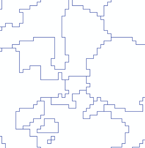
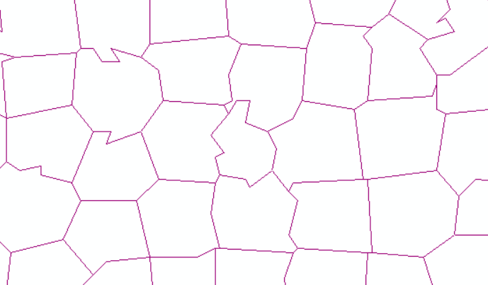
This is very interesting, English is’ multipart to singleparts’, the reason for this is that, due to the use of segmentation (segmentation) later polygonized will lead to serious jagged ‘shapefile polygon to polyline’.. When Multipolyline simplifying, the shapefile features are discrete, which leads to different States of each feature, resulting in more complexity after simplification.
The first solution is to do a cascade (Cascade), but the ogr-based cascade is done iteratively, and python is very slow in the polyline of multi-node wkt, which eventually leads to the failure of the loop, so we have to find another solution. Holding the idea of not building wheels, first of all, of course, is the industry leader in vector processing geopandas. Second, in geopandas, it is easy to find a solution. As mentioned above, after using ‘multipart to single parts’, multiple features will become single features, that is to say, they are combined and become single attributes. Then the polygon of the region is obtained by generating the range Extend of the vector, and finally the wkt is obtained by finding the intersection multipolyline. The technical route is as follows:

Because the grid can not be directly converted to a line, the first two steps here are a compromise. The third step is to find the intersection of the study area and the vector line, which is actually to find an overall feature, which is also a transformation idea.
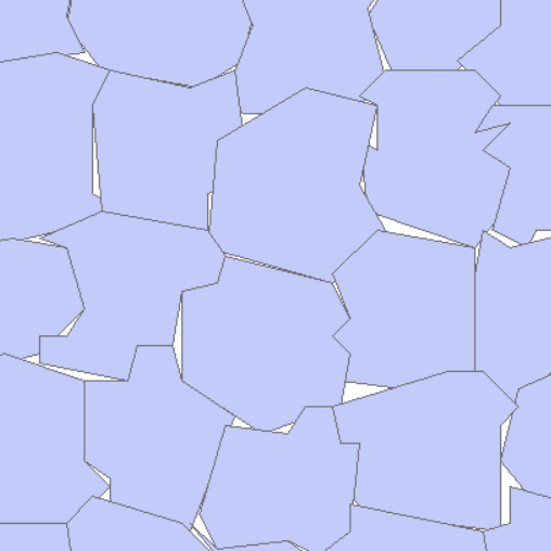
When the polyline of a single feature is simplified, there is no clutter. Here, many turning points are simplified due to the large value of the simplification tolerance (tolerance). The actual tolerance value should be set and adjusted according to its resolution value.
Speaking of the basic principles, in fact, there should be a general idea. The implementation code is directly implemented through the simplify function of geopandas, and the pre-processing function is also given here.
 1
 2
 3
 4
 5
 6
 7
 8
 9
10
11
|
def merge_all_feature_in_one(input,output):
    print("开始合并feature")
    gdf = gpd.read_file(input)
    geom = gdf['geometry']
    new_geom = gpd.tools.collect(geom)
    df = {'id': [0], 'geometry': [new_geom]}
    new_gdf = gpd.GeoDataFrame(df, crs="EPSG:4326")
    new_gdf.to_file(output)
    print("合并完成")
|
This is also achieved mainly through the collect function of geopandas.
This is a simplification function, which can also be used as a face simplification.
1
2
3
4
|
def simplifyshp(input, output, tolerance):
    gdf_main = gp.read_file(input)
    simp = gdf_main.simplify(tolerance=tolerance , preserve_topology=True)
    simp.to_file(output)
|
Orthorectified images often have a certain rotation angle in the projection space, which can be clearly seen in ENVI. Some experiments need to extract the effective range of the image. The general idea should be to get four corner points through the six parameters (Geotransform) of gdal, but is this actually accurate? Perhaps it is accurate before orthographic correction. To say the least, orthographic correction is actually the last processing step. It is theoretically no problem to extract the effective area before this step. However, some parts of the project need to be orthorectified first. Here I will continue to discuss the idea of orthorectification first. After the orthographic correction, the six parameters are not the corners of the corresponding effective area. What should we do? I have designed a binary extraction idea here. First, the image is binarized, with 1 as the segmentation point, 1 below is 0, and above is 1. After binarization, it is polygonized selected according to the attribute value of polygon. The active area of that image can be obtain.
Then the binarization function is given first:
 1
 2
 3
 4
 5
 6
 7
 8
 9
10
|
def raster_binary(input_raster,out_raster):
    dataset = gdal.Open(input_raster)
    im_width = dataset.RasterXSize
    im_height = dataset.RasterYSize
    im_geotrans = dataset.GetGeoTransform()
    im_proj = dataset.GetProjection()
    im_data = dataset.ReadAsArray(0, 0, im_width, im_height)
    ret, border0 = cv2.threshold(im_data, 0, 1, cv2.THRESH_BINARY)
    write_img(out_raster, im_proj, im_geotrans, border0)
    del dataset
|
Where the auxiliary function write_img is as follows:
 1
 2
 3
 4
 5
 6
 7
 8
 9
10
11
12
13
14
15
16
17
18
19
20
21
22
23
24
25
26
27
|
def write_img(filename, im_proj, im_geotrans, im_data):
    if 'int8' in im_data.dtype.name:
        datatype = gdal.GDT_Byte
    elif 'int16' in im_data.dtype.name:
        datatype = gdal.GDT_UInt16
    else:
        datatype = gdal.GDT_Float32

    if len(im_data.shape) == 3:
        im_bands, im_height, im_width = im_data.shape
    else:
        im_bands, (im_height, im_width) = 1, im_data.shape

    driver = gdal.GetDriverByName("GTiff")
    dataset = driver.Create(filename, im_width, im_height, im_bands, datatype)

    dataset.SetGeoTransform(im_geotrans)
    dataset.SetProjection(im_proj)
    if im_bands == 1:
        dataset.GetRasterBand(1).WriteArray(im_data)
    else:
        for i in range(im_bands):
            dataset.GetRasterBand(i + 1).WriteArray(im_data[i])

    del dataset
|
Through the binary image, take the raster to vector polygon:
 1
 2
 3
 4
 5
 6
 7
 8
 9
10
11
12
13
14
15
16
|
def PolygonizeTheRaster_bina(inputfile,outputfile):
    dataset = gdal.Open(inputfile, gdal.GA_ReadOnly)
    srcband=dataset.GetRasterBand(1)
    im_proj = dataset.GetProjection()
    prj = osr.SpatialReference()
    prj.ImportFromWkt(im_proj)
    drv = ogr.GetDriverByName('ESRI Shapefile')
    dst_ds = drv.CreateDataSource(outputfile)
    dst_layername = 'out'
    dst_layer = dst_ds.CreateLayer(dst_layername, srs=prj)
    dst_fieldname = 'DN'
    fd = ogr.FieldDefn(dst_fieldname, ogr.OFTInteger)
    dst_layer.CreateField(fd)
    dst_field = 0
    gdal.Polygonize(srcband, None, dst_layer, dst_field)
|
Create a new shapefile by selecting the feature whose ‘DN’ value field of the shapefile polygon is 1 to complete the extraction of the effective area:
 1
 2
 3
 4
 5
 6
 7
 8
 9
10
11
12
13
14
15
16
17
18
19
20
21
22
23
24
25
26
|
def SelectByAttribute(InShp, outShp):
    ds = ogr.Open(InShp,0)
    layer = ds.GetLayer(0)
    driver = ogr.GetDriverByName("ESRI Shapefile")
    ds_new = driver.CreateDataSource(outShp)
    spatialref_new = osr.SpatialReference()
    spatialref_new.ImportFromEPSG(4326)
    geomtype = ogr.wkbPolygon
    layer_new = ds_new.CreateLayer(outShp, srs=spatialref_new, geom_type=geomtype,)
    layer_new.CreateField(ogr.FieldDefn('DN', ogr.OFTInteger))
    attriNames =  ogr.OFTInteger
    features = [1]
    for i in range(layer.GetFeatureCount()):
        feature = layer.GetFeature(i)
        geom_polygon = feature.GetGeometryRef()
        name = feature.GetField('DN')
        feat = ogr.Feature(layer_new.GetLayerDefn())

        if name in attriNames:
            feat.SetGeometry(geom_polygon)
            feat.SetField('DN', name)
            features.append(feat)
    for f in features:
        layer_new.CreateFeature(f)
    ds.Destroy()
    ds_new.Destroy()
|
Obtaining the common area of the two image
This is even simpler. In fact, in vector logic, it is to find the intersection, which can be easily achieved through geopandas or other SHP processing packages. However, geopandas is based on the aggregation of other SHP processing packets and should theoretically have better processing performance.
1
2
3
4
5
|
def get_intersect_shp(out_shp_ring1 , out_shp_ring2, outshp_intersect):
    gdf_left = gpd.read_file(out_shp_ring1)
    gdf_right = gpd.read_file(out_shp_ring2)
    gdf_intersect = gpd.overlay(gdf_left,gdf_right,'intersection')
    gdf_intersect.to_file(outshp_intersect)
|
The two inputs here should be used as the two shps of the input after the effective range of the image is calculated according to the previous section of the article.
Other functions
In addition to the above several main functions, but also to do some very chicken rib function, but in some of these may inspire you, so one by one to introduce.
Cutting, needless to say, can be easily achieved based on gdal:
 1
 2
 3
 4
 5
 6
 7
 8
 9
10
|
def clip_raster_from_intersect(input_main_raster, input_shp, output_raster):
    input_raster=gdal.Open(input_main_raster)
    ds = gdal.Warp(output_raster,
                input_raster,
                format = 'GTiff',
                cutlineDSName = input_shp,
                cutlineWhere="FIELD = 'whatever'",
                dstNodata = -9999)
    ds=None
|
If you want to get the four corners of the effective range of the image, what should you do. In fact, after the SHP of the effective area is obtained as above, the corner coordinates can be easily obtained by using the extend of the SHP, and the corner function is given here.
 1
 2
 3
 4
 5
 6
 7
 8
 9
10
11
12
13
14
15
16
|
def get_extends(intersect_shp, out_shp_point):
    inDriver = ogr.GetDriverByName("ESRI Shapefile")
    inDataSource = inDriver.Open(intersect_shp, 0)
    inLayer = inDataSource.GetLayer()
    corners = inLayer.GetExtent()
    point1 =  geometry.Point(corners[0,0],corners[1,0])
    point2 =  geometry.Point(corners[0,1],corners[1,1])
    point3 =  geometry.Point(corners[0,3],corners[1,3])
    point4 =  geometry.Point(corners[0,2],corners[1,2])
    pointshp = gpd.GeoSeries([point1, point2, point3, point4],
                                crs='EPSG:4326',  # 指定坐标系为WGS 1984
                                index=['0', '1']  # 相关的索引
                                )
    pointshp.to_file(out_shp_point,driver='ESRI Shapefile',encoding='utf-8')
    inDataSource = None
    out_shp_point = None
|
You can actually write a dictionary here, or list to iteratively import geometry, but there are only four corners in the range, so you are too lazy to write a loop.
In fact, there is also an ogr version of simplification, or smoothing. The principle is to build a buffer line through the buffer to complete the smoothing curve. However, this is not feasible in multiple features, that is, there will be line superposition after simplification. As mentioned in the previous article, here is also a reference. This function is written by someone else, so I will not discuss it.
 1
 2
 3
 4
 5
 6
 7
 8
 9
10
11
12
13
14
15
16
17
18
19
20
21
22
23
24
25
26
27
28
|
def smoothing(inShp, fname, bdistance=2):
    """
    :param inShp: 输入的矢量路径
    :param fname: 输出的矢量路径
    :param bdistance: 缓冲区距离
    :return:
    """
    ogr.UseExceptions()
    in_ds = ogr.Open(inShp)
    in_lyr = in_ds.GetLayer()
    # 创建输出Buffer文件
    driver = ogr.GetDriverByName('ESRI Shapefile')
    if Path(fname).exists():
        driver.DeleteDataSource(fname)
    # 新建DataSource,Layer
    out_ds = driver.CreateDataSource(fname)
    out_lyr = out_ds.CreateLayer(fname, in_lyr.GetSpatialRef(), ogr.wkbMultiLineString)
    def_feature = out_lyr.GetLayerDefn()
    # 遍历原始的Shapefile文件给每个Geometry做Buffer操作
    for feature in tqdm.tqdm(in_lyr):
        geometry = feature.GetGeometryRef()
        buffer = geometry.Buffer(bdistance,1).Buffer(-bdistance,1)
        out_feature = ogr.Feature(def_feature)
        out_feature.SetGeometry(buffer)
        out_lyr.CreateFeature(out_feature)
        out_feature = None
    out_ds.FlushCache()
    del in_ds, out_ds
|
There is also a logical sum, but this is basically useless. For a vector file with multiple features and strict contact between features, using it will cause all the features to merge into a large SHP block, but all the wkt points are gone, which is the real meaning of fusion. I forgot to cut the screenshot of the specific experimental SHP file. Interested readers can do their own experiments.
 1
 2
 3
 4
 5
 6
 7
 8
 9
10
11
12
13
14
15
16
17
18
19
20
21
22
23
24
25
26
27
28
29
30
31
32
33
|
def uni(shpPath, fname):
    """
    :param shpPath: 输入的矢量路径
    :param fname: 输出的矢量路径
    :return:
    """
    driver = ogr.GetDriverByName("ESRI Shapefile")
    dataSource = driver.Open(shpPath, 1)
    layer = dataSource.GetLayer()

    # 新建DataSource,Layer
    out_ds = driver.CreateDataSource(fname)
    out_lyr = out_ds.CreateLayer(fname, layer.GetSpatialRef(), ogr.wkbLineStringZM)
    def_feature = out_lyr.GetLayerDefn()
    # 遍历原始的Shapefile文件给每个Geometry做Buffer操作
    current_union = layer[0].Clone()
    print('the length of layer:', len(layer))
    if len(layer) == 0:
        return

    for i, feature in tqdm.tqdm(enumerate(layer)):
        geometry = feature.GetGeometryRef()
        if i == 0:
            current_union = geometry.Clone()
        current_union = current_union.Union(geometry).Clone()

        if i == len(layer) - 1:
            out_feature = ogr.Feature(def_feature)
            out_feature.SetGeometry(current_union)
            out_lyr.ResetReading()
            out_lyr.CreateFeature(out_feature)
|
In addition, gdal has two summation functions, one is normal Union, the other is cascade UnionCascaded, but I can’t see the difference between the two. In fact, cascade is also recommended by a group friend. In the end, I didn’t get the ideal result. Here is the code of cascade.
1
2
3
4
5
6
7
|
def dedup(geometries):
    """Return a geometry that is the union of all geometries."""
    if not geometries:  return None
    multi  = ogr.Geometry(ogr.wkbMultiPolygon)
    for g in geometries:
        multi.AddGeometry(g.geometry())
    return multi.UnionCascaded()
|
In fact, the above corner coordinates are used to determine the farthest point of the effective area. In order to achieve this goal, I also built a wheel in the early stage. As a result, the wheel is not rigorous enough. Maybe it can run through this image, but not the other one. The main idea is to find the nearest value point by iterating the farthest line around the center of the image. The initial value point in four directions is defined as the farthest possible point, and then the farthest two points are solved by calculating the distance and judging. However, the effective points between some image bands do not necessarily conform to my judgment definition, and for many other complex reasons, this function is abandoned, but here it is released to the reader, hoping to give the reader some inspiration.
 1
 2
 3
 4
 5
 6
 7
 8
 9
10
11
12
13
14
15
16
17
18
19
20
21
22
23
24
25
26
27
28
29
30
31
32
33
34
35
36
37
38
39
40
41
42
43
44
45
46
47
48
49
50
51
52
53
54
55
56
57
58
59
60
61
62
63
64
65
66
67
68
69
70
71
72
73
|
def get_start_end_points(in_raster, out_shp_point):
    ogr.RegisterAll()
    dataset = gdal.Open(in_raster)
    geocd = dataset.GetGeoTransform()
    row = dataset.RasterXSize #hang
    line = dataset.RasterYSize #lie
    band1=dataset.GetRasterBand(1)
    im_datas1 = band1.ReadAsArray(0, 0, row, line)
    im_datas1 = im_datas1.transpose((1,0))
    for i in range(row):
        if im_datas1[0,i] != 0:
            lefttopx = geocd[0]
            lefttopy = geocd[3] + i * geocd[5]
            print(im_datas1[0,i])
            break
        elif im_datas1[1,i] != 0:
            lefttopx = geocd[0] + 1 * geocd[1]
            lefttopy = geocd[3] + i * geocd[5]
            print(im_datas1[1,i])
            break

    for i in range(row):
        if im_datas1[row-1,i] != 0:
            rightdownx = geocd[0] + row * geocd[1]
            rightdowny = geocd[3] + i * geocd[5]
            print(im_datas1[row-1,i])
            break
        elif im_datas1[row-2,i] != 0:
            rightdownx = geocd[0] + (row-1) * geocd[1]
            rightdowny = geocd[3] + i * geocd[5]
            print(im_datas1[row-2,i])
            break

    for i in range(line):
        if im_datas1[i,0] != 0:
            leftdownx = geocd[0] + i * geocd[1]
            leftdowny = geocd[3]
            print(im_datas1[i,0])
            break
        elif im_datas1[i,1] != 0:
            leftdownx = geocd[0] + i * geocd[1]
            leftdowny = geocd[3] + 1 * geocd[5]
            print(im_datas1[i,1])
            break

    for i in range(line):
        if im_datas1[i,line-1] != 0:
            righttopx = geocd[0] + i * geocd[1]
            righttopy = geocd[3] + line * geocd[5]
            print(im_datas1[i,line-1])
            break
        elif im_datas1[i,line-2] != 0:
            righttopx = geocd[0] + i * geocd[1]
            righttopy = geocd[3] + (line-1) * geocd[5]
            print(im_datas1[i,line-2])
            break

    if  row <= line:
        start = geometry.Point(leftdownx, leftdowny)
        end = geometry.Point(righttopx, righttopy)

    else:
        start = geometry.Point(lefttopx, lefttopy)
        end = geometry.Point(rightdownx, rightdowny)

    pointshp = gpd.GeoSeries([start, end],
                            crs='EPSG:4326',  # 指定坐标系为WGS 1984
                            index=['0', '1']  # 相关的索引
                            )
    pointshp.to_file(out_shp_point,driver='ESRI Shapefile',encoding='utf-8')
    del dataset
|
However, this function was written out and abandoned, which also taught me a profound lesson-if you can’t build a wheel, you can’t build it, which really needs to be remembered.
Postscript
The big lesson is to refuse to build wheels. Then the geopandas is really strong, rarely used before, but this use gave me a very deep impression, as expected, standing on the shoulders of giants, or see far. In fact, I also found some shapefile polyline simplification algorithms that go deep into the principle layer, but as an engineering implementation, the stability is still the first one I use, and the stability of geopandas is needless to say. For the rest, write about it in a future article.