Yikang (eCognition) software is familiar to those who are familiar with object-oriented classification of remote sensing. It is a very good object-oriented classification software developed by several old German engineers, which can be used for object-oriented classification of multi-spectral images such as medicine and remote sensing.

In fact, object-oriented classification is called Object-based Image Analysis (OBIA) in academia, while in remote sensing and other geoscience subdivisions, it is called Geo-Object-based Image Analysis (GEOBIA), which has obvious advantages. Different from the ordinary iterative classification of pixel violence, the concept of object is embodied in the collection of homogeneous pixels, which can remove the “salt and pepper effect” to a great extent, different from the effect of fuzzy classification, its object boundary is obvious.

Image segmentation is the most important part of object-oriented processing. The existing image segmentation algorithms mainly include watershed, SLIC, quickshift and classical Graphcut, etc. According to the different uses, the first three will be used in the subdivision field, for example, watershed and SLIC are mostly used in medicine, quickshift is mostly used in remote sensing, followed by SLIC.

In fact, ecognition has well met the needs of the existing research foreword. I don’t know how many articles have been written, but the key is that it is commercial software. Although it can be cracked, as an open source GIS enthusiast, it should be a small wish to be able to write its open source solution. In this segmentation, I use a small data cut out by myself, mainly to save time and facilitate writing articles.

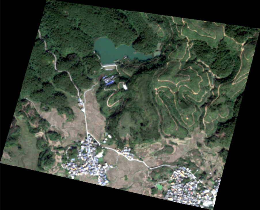
There are water, vegetation, bare land and building land in the region, and the basic categories are all complete, which should be good experimental data.

Segmentation algorithm

Let’s start with two of the segmentation algorithms I use.

SLIC segmentation is based on the segmentation results of the number of seeds, according to the set number of super-pixels, the seed points are evenly distributed in the image. Therefore, the number of seeds is the key to the effect and speed of image segmentation. The more the number, the finer the segmentation, and the longer the segmentation time. However, in recent experiments, it has been found that the number of seeds does not have much impact on time, while the number of pixels has much greater impact than the previous indicators. When the pixel number is 10000 * 10000, the segmentation time reaches 5 minutes when the number of seeds is 10000. Of course, this is not a very rigorous experimental data, but also need to do a few more experiments to get the law. SLIC is already integrated in the scikit-image Python package, so it’s not a problem to write it yourself, but it’s not advisable to build wheels. There are many parameters in this algorithm, but the main ones are the number of segmentation seeds and compactness, where compactness indicates the optional balance of color proximity and spatial proximity. The higher the value, the heavier the spatial proximity, which makes the shape of the superpixel more square/cubic. This parameter is generally divided by 10 times the size of the float in the general case of parameter adjustment..g. 0.01, 0.1, 1, 10, 100. Other parameters are set as required and will not be repeated here.

Quickshift is a fast displacement clustering algorithm, which is also a very powerful segmentation algorithm. Based on the approximation of the average movement of the kernel, it can calculate the hierarchical segmentation at multiple scales, and to some extent, it has a miraculous effect on the scale effect of remote sensing. There are two or three most important parameters of quickshift. One is ratio, which is between 0 and 1 to balance the closeness of color space and image space. A higher value will increase the weight of color space. Kernel _ size is a Gaussian kernel width that can be chosen to smooth the sample density. Higher means fewer clusters. Max _ dist is the tangent point for the optional data distance. Higher means fewer clusters.

Now let’s take a look at the effect of processing remote sensing TIF images with scikit-image packets. The code is as follows:

 1
 2
 3
 4
 5
 6
 7
 8
 9
10
11
12
13
14
15
16
17
18
19
20
21
22
23
24
25
26
27
28
29
30
31
32
33
34
35
36
37
38
39
40
41
42
43
44
45
46
47
48
49
50
51
52
53
54
55

from skimage.segmentation import mark_boundaries
from osgeo import  gdal
from skimage.segmentation import  slic, quickshift


def read_img(filename):
    dataset = gdal.Open(filename)
    im_width = dataset.RasterXSize
    im_height = dataset.RasterYSize
    im_geotrans = dataset.GetGeoTransform()
    im_proj = dataset.GetProjection()
    im_data = dataset.ReadAsArray(0, 0, im_width, im_height) #0, 0, im_width, im_height
    del dataset
    return im_width, im_height, im_proj, im_geotrans, im_data


def write_img(filename, im_proj, im_geotrans, im_data):
    if 'int8' in im_data.dtype.name:
        datatype = gdal.GDT_Byte
    elif 'int16' in im_data.dtype.name:
        datatype = gdal.GDT_UInt16
    else:
        datatype = gdal.GDT_Float32

    if len(im_data.shape) == 3:
        im_bands, im_height, im_width = im_data.shape
    else:
        im_bands, (im_height, im_width) = 1, im_data.shape

    driver = gdal.GetDriverByName("GTiff")
    dataset = driver.Create(filename, im_width, im_height, im_bands, datatype)

    dataset.SetGeoTransform(im_geotrans)
    dataset.SetProjection(im_proj)
    if im_bands == 1:
        dataset.GetRasterBand(1).WriteArray(im_data)
    else:
        for i in range(im_bands):
            dataset.GetRasterBand(i + 1).WriteArray(im_data[i])

    del dataset
    
    
img_path = r".\test.tif"
temp_path = r".\classification"
im_width, im_height, im_proj, im_geotrans, im_data = read_img(img_path)
im_data = im_data[0:3]
temp = im_data.transpose((2, 1, 0))
#segments_quick = quickshift(temp, kernel_size=3, max_dist=6, ratio=0.5)
segments_quick = slic(temp, n_segments=25000, compactness=10.)
mark0 = mark_boundaries(temp, segments_quick)
save_path = temp_path + "temp.tif"
re0 = mark0.transpose((2, 1, 0))
write_img(save_path, im_proj, im_geotrans, re0)

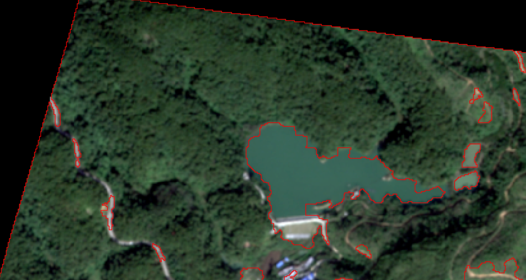
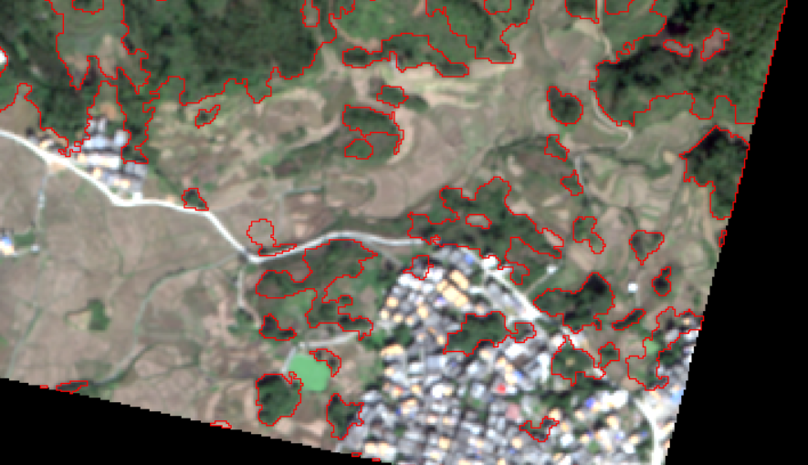
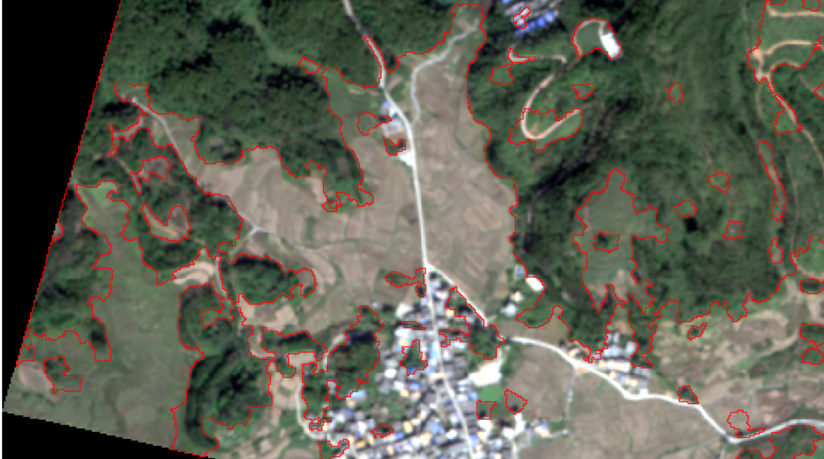
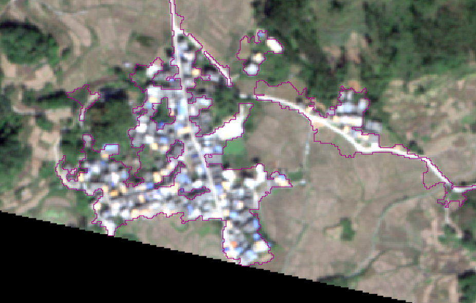
It returns a two-dimensional array, and the pixel value of each cluster block is the same, but this value only represents the order of the block, and does not represent any remote sensing or physical meaning. You can call these values IDs. These ID values are also important values for subsequent positioning in two-dimensional space. Take a quick look at what these segmented images look like:

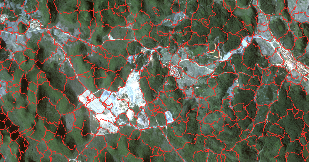
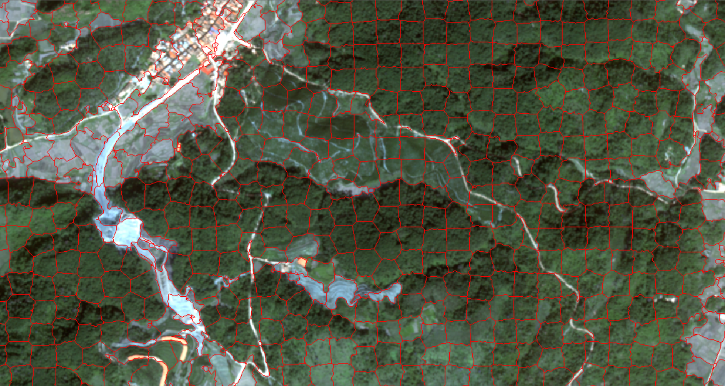
Of course, after the code is executed, the output is actually a raster TIF, but the raster file is not easy to view, so I converted the raster into a vector line and superimposed it on the original multi-spectral remote sensing image, so that readers can roughly feel the segmentation situation.

Land type data

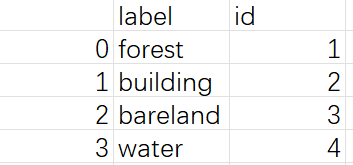
The data of ground object category is made by myself with arcmap. After the image is cropped to 700 * 500 pixels, the image is simply divided into several categories according to visual observation:

1. Woodland
2. Bare ground
3. Architecture
4. Waters

According to the machine learning convention, the label data needs to be split into a test set and a validation set. The ratio is 7:3, which can be easily achieved by using geopandas. The code is as follows:

 1
 2
 3
 4
 5
 6
 7
 8
 9
10
11
12

gdf = gpd.read_file(r".\sub_sample.shp")
class_names = gdf['label'].unique()
class_ids = np.arange(class_names.size) + 1
df = pd.DataFrame({'label': class_names, 'type': class_ids})
df.to_csv(r".\temp.csv")
gdf['type'] = gdf['label'].map(dict(zip(class_names, class_ids)))
gdf_train = gdf.sample(frac=0.7)  
gdf_test = gdf.drop(gdf_train.index)
gdf_train.to_file(r".\train_data1.shp")
gdf_test.to_file(r".\test_data1.shp")

Build features

As the old saying goes, creating new features is a very difficult thing, requiring a lot of expertise and a lot of time. The essence of machine learning applications is basically feature engineering. ——Andrew Ng

As an object-oriented classification of remote sensing, the number of optional features can reach hundreds, generally including various vegetation indices, mean, variance, standard deviation, gray level co-occurrence matrix, etc., and other researchers use other data such as phenology, temperature and so on to participate in feature construction, and then optimize the features, and finally put the features into the random forest training machine for classification. The focus of this experiment is on the python implementation, so there are not too many features built, and a small number of features means that there is no need for feature optimization, which saves a lot of steps.

It is worth mentioning that in the feature construction step, it takes tens of times longer than the segmentation, so if the image is very large, it needs to write multi-threading to speed up the feature construction process. In the image of 10000 * 10000 pixels, the training time of only three features reached 1.5 hours.

 1
 2
 3
 4
 5
 6
 7
 8
 9
10
11
12
13
14
15
16
17
18
19
20

def segment_features(segment_pixels):
    features = []
    npixels, nbands = segment_pixels.shape
    for b in range(nbands):
        stats = scipy.stats.describe(segment_pixels[:, b])
        band_stats = list(stats.minmax) + list(stats)[2:]
        if npixels == 1:
            band_stats[3] = 0.0
        features += band_stats
    return features


segment_ids = np.unique(segments)
objects = []
object_ids = []
for id in segment_ids:
    segment_pixels = temp[segments == id]
    object_features = segment_features(segment_pixels)
    objects.append(object_features)
    object_ids.append(id)

Land type vector to grid

This step is to make the land class value and the object of the image fall in the same area, so that the segmented object in the image can be assimilated into the actual land class.

 1
 2
 3
 4
 5
 6
 7
 8
 9
10
11
12
13
14

train_fn = r".\train_data1.shp"
train_ds = ogr.Open(train_fn)
lyr = train_ds.GetLayer()
driver = gdal.GetDriverByName('MEM')
target_ds = driver.Create('', im_width, im_height, 1, gdal.GDT_UInt16)
target_ds.SetGeoTransform(im_geotrans)
target_ds.SetProjection(im_proj)
options = ['ATTRIBUTE=tyPE']
gdal.RasterizeLayer(target_ds, [1], lyr, options=options)
data = target_ds.GetRasterBand(1).ReadAsArray()
ground_truth = target_ds.GetRasterBand(1).ReadAsArray()
ground_truth = ground_truth.transpose((1, 0))
classes = np.unique(ground_truth)[1:]

And finally obtaining the grid point data with the ground object category data.

Feature matching

After the obtained grid point real ground object data is matched with the image object through iteration, the corresponding features of the object are searched through an iterator.

 1
 2
 3
 4
 5
 6
 7
 8
 9
10
11
12
13
14
15
16
17
18
19
20
21
22
23
24
25
26
27
28
29
30
31
32
33
34
35
36
37
38

segments_per_class = {}
for klass in classes:
    segments_of_class = segments[ground_truth == klass]
    segments_per_class[klass] = set(segments_of_class)
 
intersection = set()
accum = set()
for class_segments in segments_per_class.values():
    intersection |= accum.intersection(class_segments)
    accum |= class_segments
assert len(intersection) == 0, "Segment(s) represent multiple classes"
print("adjust complete")
end3 = time.time()
print('Running time2: %s Seconds'%(end3-start3))




print("start train randomforest classification")
start4 = time.time()
train_img = np.copy(segments)
threshold = train_img.max() + 1 

for klass in classes:
    class_label = threshold + klass
    for segment_id in segments_per_class[klass]:
        train_img[train_img == segment_id] = class_label
 
train_img[train_img <= threshold] = 0
train_img[train_img > threshold] -= threshold

training_objects = []
training_labels = []
for klass in classes:
    class_train_object = [v for i, v in enumerate(objects) if segment_ids[i] in segments_per_class[klass]]
    training_labels += [klass] * len(class_train_object)
    training_objects += class_train_object

In the actual process of image sample construction, some object samples may have a small distance from each other, causing two or more samples to fall into the same segmentation area, which will lead to infinite feature matching iterations, so we need to take one of the two or more samples, which is the role of the above script.

Classification

Everything is ready. Finally, the random forest classifier is used scikit-learn to predict the sample segmentation blocks and other undefined segmentation blocks, and the results are output to the grid.

 1
 2
 3
 4
 5
 6
 7
 8
 9
10
11
12
13
14
15
16
17
18
19
20
21
22
23
24
25
26
27
28
29
30
31
32
33
34
35
36
37
38
39
40
41
42
43

def PolygonizeTheRaster(inputfile,outputfile):
    dataset = gdal.Open(inputfile, gdal.GA_ReadOnly)
    srcband=dataset.GetRasterBand(1)
    im_proj = dataset.GetProjection()
    prj = osr.SpatialReference() 
    prj.ImportFromWkt(im_proj)
    drv = ogr.GetDriverByName('ESRI Shapefile')
    dst_ds = drv.CreateDataSource(outputfile)
    dst_layername = 'out'
    dst_layer = dst_ds.CreateLayer(dst_layername, srs=prj)
    dst_fieldname = 'DN'
    fd = ogr.FieldDefn(dst_fieldname, ogr.OFTInteger)
    dst_layer.CreateField(fd)
    dst_field = 0
    gdal.Polygonize(srcband, None, dst_layer, dst_field) 

classifier = RandomForestClassifier(n_jobs=-1)  
classifier.fit(training_objects, training_labels) 
predicted = classifier.predict(objects)  

clf = segments.copy()
for segment_id, klass in zip(segment_ids, predicted):
    clf[clf == segment_id] = klass
# temp = temp.transpose((2, 1, 0))
mask = np.sum(temp, axis=2)  
mask[mask > 0.0] = 1.0   
mask[mask == 0.0] = -1.0

clf = np.multiply(clf, mask)
clf[clf < 0] = -9999.0
clf = clf.transpose((1, 0))
clfds = driverTiff.Create(r"D:\Data\testdata\classification\result.tif", im_width, im_height,
                          1, gdal.GDT_Float32) 
clfds.SetGeoTransform(im_geotrans)
clfds.SetProjection(im_proj)
clfds.GetRasterBand(1).SetNoDataValue(-9999.0)
clfds.GetRasterBand(1).WriteArray(clf)
clfds = None

end4 = time.time()
outputfile = r".\result2.shp"
print('Running time2: %s Seconds'%(end4-start4))
PolygonizeTheRaster(r".\result.tif",outputfile)

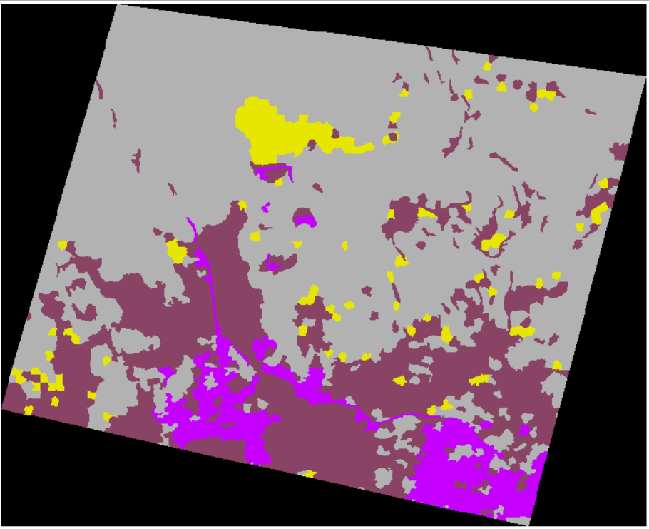
Of course, because of the above reasons, the tag ID classified in the image is 1, 2, 3 and so on, so it is difficult to view with the naked eye with the general grid viewing software. Here, in order to facilitate the reader to view and draw, I also carried out the operation of grid to vector, so that the classification can be clearly viewed in arcmap.

Final classification results:

Look at the details again:

In terms of forest land, the classification is generally perfect.

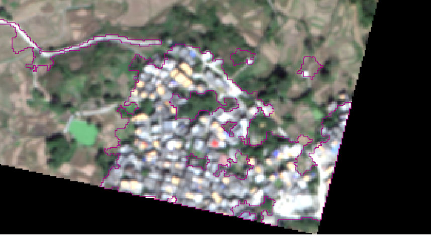
It also has a good classification effect on human activity areas.

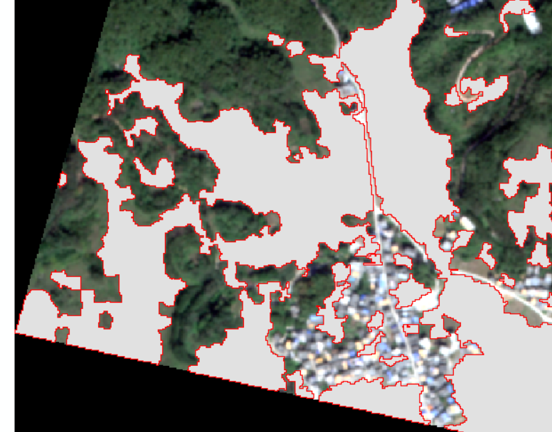The bare ground is also great.

The classification effect of 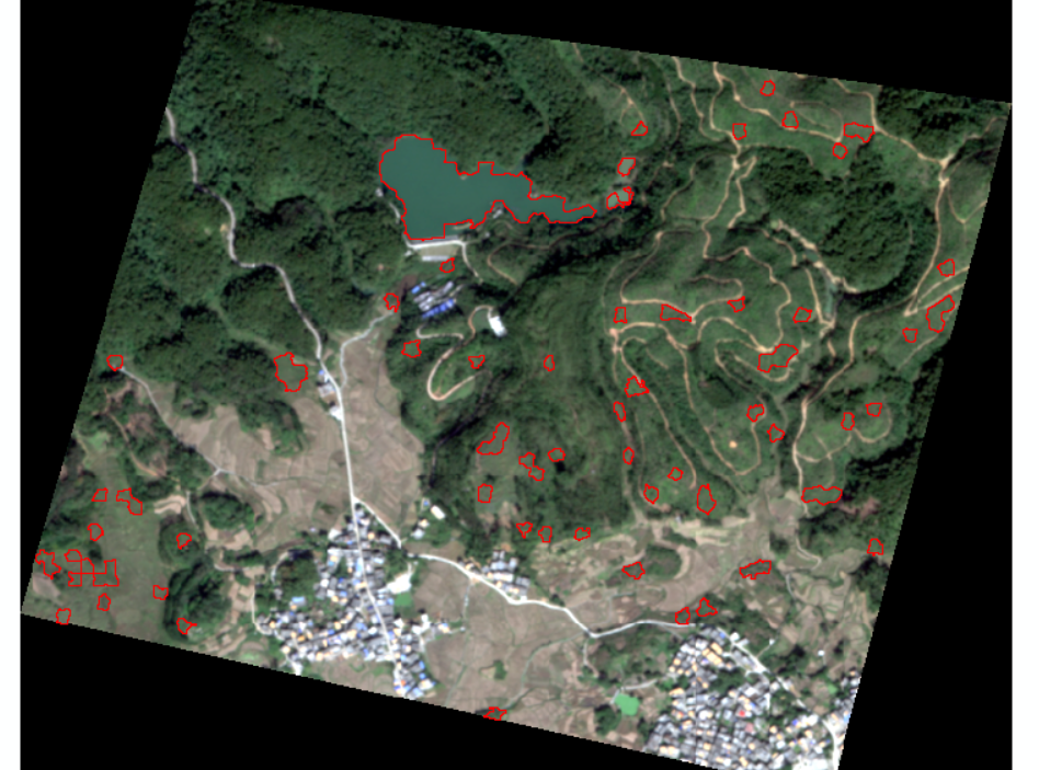water system is very poor, which may be due to insufficient characteristics.

Conclusion

Generally speaking, the classification results are good. On the one hand, the study area is small, and on the other hand, I have selected enough sample points. At present, I have not tried to classify on large images. My notebook only needs one and a half hours for feature construction, which is really impossible.

Object-oriented classification is one of the contents that the undergraduate junior has been studying with the teacher. It was originally to explore the fit point of scale effect and multi-scale segmentation. However, as time goes on, it fails to produce any good results. It will use Yikang to keep adjusting parameters and experimenting. Sometimes it is normal to adjust to two or three o’clock in the middle of the night. It’s a pity that I didn’t learn python well at that time, and I couldn’t make good use of the existing resources to carry out experiments efficiently, otherwise I might have a good paper again.

But this is also a wish, has been very grateful to the undergraduate teachers for their careful training, the open source implementation of this algorithm, means that this experiment can be put aside today. The next technical article may focus more on sharing the experience of deep learning semantic segmentation network.